Lesson 12 Linking and Protecting your worksheet
This week you will return to the textbook and familiarize yourself with the step-by-step exercises in Lesson 12.
There is short submission this week from the book, page 541 which I will type up for those who do not have the book.
The protection schemes available go beyond simply locking the entire worksheet as indicated in the book. Investigate the Formatting of cells to lock only some cells (see this lecture). Use the discussion board for more information.
Below is a summary of linking to internal sheets as well as external files.
Topics this week included:
Linked Formulas
The purpose of linking is to replace the usual copy and paste with linking, so that any change in the original or source data, will automatically update on all the destination locations! It is also used to pull data from several worksheets into separate worksheet.
Linking to different sheets or workbooks is a simple concept. It is sometimes referred to as consolidating data. When we use more than one sheet or workbook, and have the need to pull data from several places into one, simply reference the cell that contains the desired data by referring not just to the cell address, such as A1, but designate which A1, as in Sheet1!A1. For too long we have been using only one sheet in our projects and might have forgotten that when we say A1, that there are many A1s.
The image below shows Hours Worked for each employee, for Week1 on Sheet1. Imagine a similar layout for hours worked for week 2, week 3 and week 4.
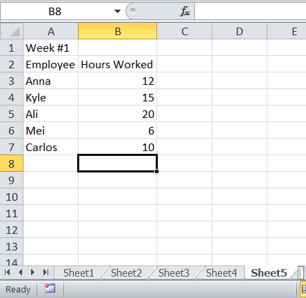
Now on Sheet 5 we would like to total the hours for each employee. A complete formula in Sheet 5, that sums up all the data in cells A1 of Sheets 1 through 4, might look like this:
=Sheet1!B3+Sheet2!B3+Sheet3!B3+Sheet4!B3
This formula can be anywhere on Sheet5 and would reflect the sum of all the data in cells B3 of sheets 1 through 4.
To create this formula without typing it in, you can simply start by typing the = into the desired cell of Sheet5 and then beginning pointing to each cell on the previous sheets that you want to include in the formula. Press <enter> when done and the formula will appear in Sheet5. If the Names should also be linked, then perhaps the names should be typed in only on Sheet1 and in all other sheets a formula like this would link to the name: =Sheet1!A3
Copying these formulas down will take care of all the names and totals.
If the layout of all the sheets is exactly the same, meaning the data to add is in cell A1 of all the sheets, a more efficient formula could be constructed by typing =SUM( in the desired cell of sheet5, select Sheet1, select A1, hold the <shift> and click Sheet4 tab, press <enter>. The resulting formula on Sheet5 will look like this:
=SUM(Sheet1:Sheet4!B3)
An alternative typing in this formula or using the pointing method, you can also use the Tool Ribbon. Select the destination cell on Sheet5, then choose the Data tab, then the Consolidate tool.
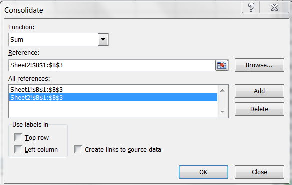
Select the ranges to sum, use the add button before reaching for another range. Once you click OK, the sum results will appear in the currently selected cell but no formula will be there so no automatic updating will take place, unless you click the Create Links to Source Data check box.
Remember you can also name your sheets for clarity, before or after the formula is constructed:
=Qtr1!A1+Qtr2!A1+Qtr3!A1+Qtr4!A1
=SUM(Qtr1:Qtr4!A1)
Sometimes it is handy to see all the sheets at the same time. This can only be accomplished if the sheets are first placed into their own window. Use the tool ribbon to select View and then click the New Window as many times as you have sheets to display. Then on the tool ribbon, click Arrange All, then choose Tile. The file name will be followed by a : (colon) and a number to indicate the window number.
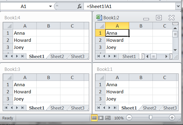
You can now choose to view different sheets in each tiled window.
In the graphic above, the tile titled Book1:2 has been set to show Sheet2 while all the other tiles remain on Sheet1. Notice the formula in cell A1 of Book1:2. This way we don't type the names over and over on each sheet. The value of this linked formula is that any change of the spelling of the name on Sheet1, will cascade on all the sheets where the linked formula appears. An alternative to typing the formula, you can use Copy and Paste Special, and then Paste Link for the exact same result.
To return to normal view, just randomly close all but one window.
One warning about using linked cells: Sorting can be an issue as data in some columns are tied to a master sheet and juggling the rows during a sort can be disastrous. The only way to get around this is to replace the linked formulas with absolute references!
The method to link across completely separate files or workbooks, is the same but the resulting formulas are understandably more complex as the cell reference must include not just the sheet name but the filename as well. In addition, when the file that is linked to, is closed, the formula expands to include the file path!
=[file4.xlsx]Sheet1!$B$1+[file3.xlsx]Sheet1!$B$1+[file1.xlsx]Sheet1!$B$1 etc.
When the linked files are closed, the formula changes to this horror:
='C:\Users\Terry\Documents\[file4.xlsx]Sheet1'!$B$1+'C:\Users\Terry\Documents\[file3.xlsx]
Sheet1'!$B$1 etc.
Also, when the pointing method is used across different files or workbooks, the default cell reference is for absolute. You can choose to remove this for ease in copying down the formula.
This works across applications as well
Try copying a simple range of student names and Test scores to a Word document. If you use the normal copy and paste method, changes in the Excel sheet will not be reflected in the Word document. Try instead to use copy, switch to Word and use Paste, Paste Special, Paste Link.
Now that you know the details of linking formulas, let's explore a step-by-step use of the Tool Ribbon to accomplish this in a more streamlined way. This approach only works if the layout of the sheets to be consolidated, are exactly the same, or in another case, at least have the same labels.
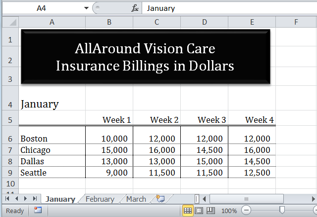
Imagine an exact layout for the February and March sheets and we need to consolidate all the data for the first quarter on Sheet4.
Start by copying and pasting one of the sheets on Sheet4 and deleting the numeric data and labeling A4, Summary.
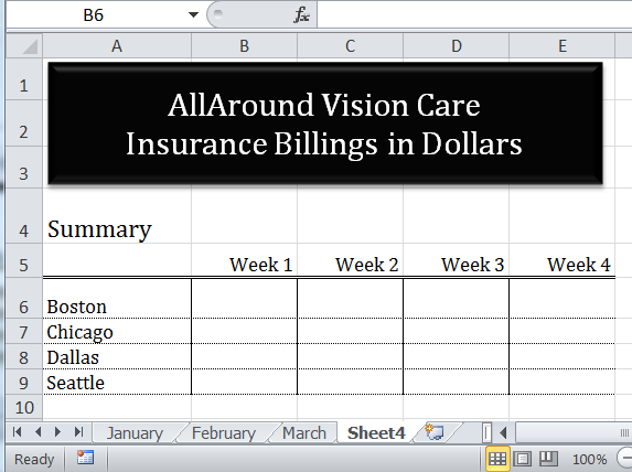
Now with B6:E9 selected, click Data, Consolidate on the Ribbon. Choose the Sum function. In the reference box as shown below, click the January tab, and select the range B6:E9. Click Add to add the reference to the reference box.
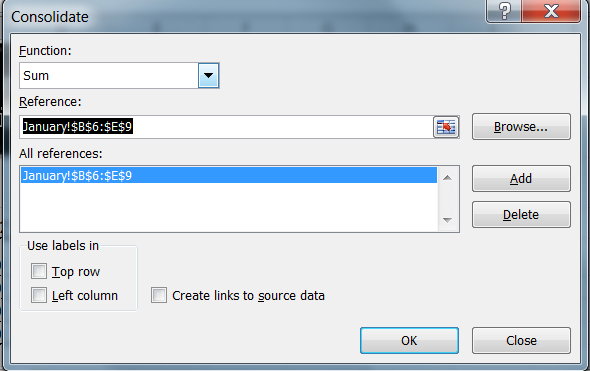
Repeat for the February and March Sheets. When you click OK. The data will be consolidated according to the function you chose (Sum in this case), but no formulas are added to Sheet4. If you want the consolidation to be be dynamic, update when changes are made to the sheets, then check the Create Links to Source date check box. The consolidation will be slightly different using an outline layout.
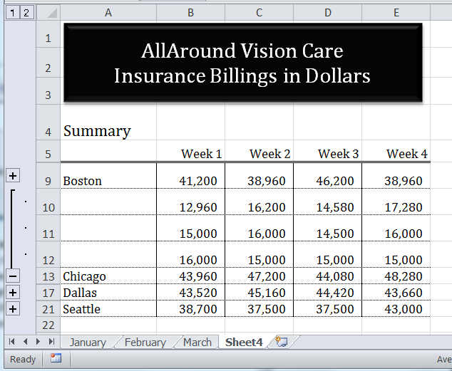
Explore by clicking the + and - symbols.
One last option addresses the situation when the layout isn't exactly the same. To explre this, jsut simply rearrange the labels so that the cities are in different positions on the different sheets. So on the January sheet, the cities might go in this order:
and the weeks might look like this:
and on the February and March sheets they would be different.
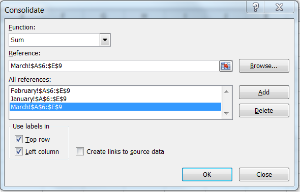
Repeat the same steps but this time in the consolidate dialog box, select the check boxes for top row and left column as shown below. Also, this time you would highlight the entire area to include the labels as well - $A$6:$E$9
Protecting and Locking Worksheet and Cells
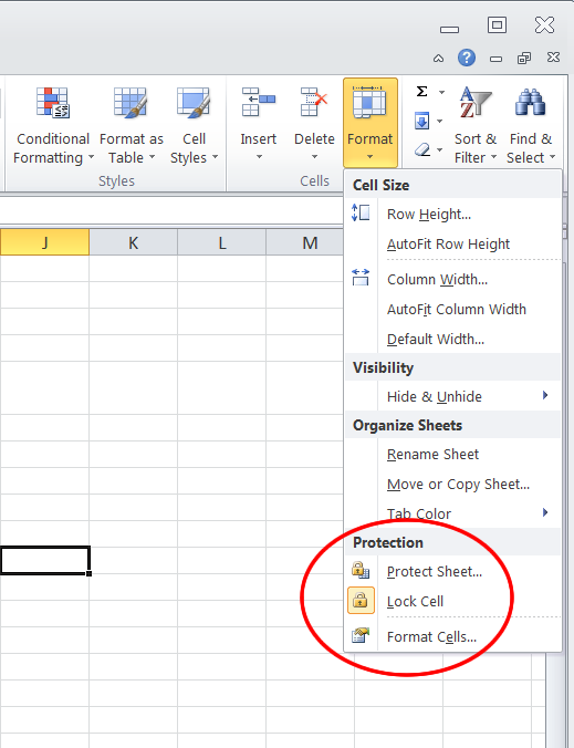
To protect an entire sheet's data from being accidentally typed over, simply select the menu option for protecting the sheet. You can find this under the Review Tab or on the Home Tab, Cell group/section as shown below.
Selecting Protect Sheet will produce this dialog box:
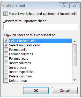
Just click OK and the entire sheet is now protected and no editing can be done in any of the cells!
To protect an entire sheet's data from being intentionally typed over, simply repeat the steps but enter a password when prompted. Yo will be asked to verify the password. As always, write down your password as there is no way to retrieve the data if you cannot remember the password. (Unless you know a hacker.)
To leave some cells unlocked for editing, the process is bit more involved and seems contrary to many people but here goes.
You may want to allow users to enter data such as customers names, Items, Quantities Ordered etc., but lock the cells with formulas. To do this, you must:
As you know by now, you can get to the dialog box shown above in many ways. One way is to select Format from the Cells group, (see first graphic in this section), and then Format Cells, then click the last tab titled Protection to see this:
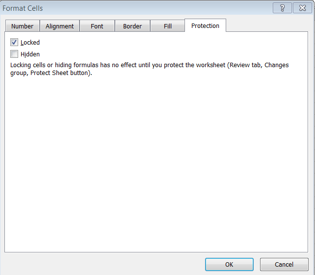
Uncheck the Locked box and click OK. (Nothing at this point is noticeably changed, but the selected cells are marked for "staying open" when the sheet is protected/locked.)
Now protect the sheet as you did before. You will now be able to type into the selected cells only!
A quick path to this is to select the cells to remain open. Now use the menu as shown in the first graphic in this section, Format, choose the option Lock Cell. This sets the format to keep these cells open. Now protect the sheet as usually done.
To hide formulas in the Formula Bar.
Select the cells with formulas. Go to the Format Dialog box for Protection as shown in the graphic above (the one with the Protect and Hide check boxes), check the Hide check box. Protect the sheet as normal. Now you will not be able to see the formulas when the cells are selected!
Preventing the file from being opened.
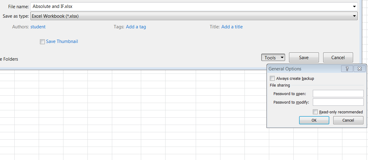
The ultimate protection is to save the file with a password. Yo can choose the save password mode to be either:
Not able to open at all
Open, but not able to modify
This is accomplished through the saving option.
Choose File, Save As, Tools, General options. See graphic below:
See you online!
Terry
This week you will return to the textbook and familiarize yourself with the step-by-step exercises in Lesson 12.
There is short submission this week from the book, page 541 which I will type up for those who do not have the book.
The protection schemes available go beyond simply locking the entire worksheet as indicated in the book. Investigate the Formatting of cells to lock only some cells (see this lecture). Use the discussion board for more information.
Below is a summary of linking to internal sheets as well as external files.
Topics this week included:
- Linking sheets within the same workbook as well as linking sheets in separate workbooks.
- Protecting or Locking worksheet and Cells
- Hiding Formulas in the Formula Bar
Linked Formulas
The purpose of linking is to replace the usual copy and paste with linking, so that any change in the original or source data, will automatically update on all the destination locations! It is also used to pull data from several worksheets into separate worksheet.
Linking to different sheets or workbooks is a simple concept. It is sometimes referred to as consolidating data. When we use more than one sheet or workbook, and have the need to pull data from several places into one, simply reference the cell that contains the desired data by referring not just to the cell address, such as A1, but designate which A1, as in Sheet1!A1. For too long we have been using only one sheet in our projects and might have forgotten that when we say A1, that there are many A1s.
The image below shows Hours Worked for each employee, for Week1 on Sheet1. Imagine a similar layout for hours worked for week 2, week 3 and week 4.
Now on Sheet 5 we would like to total the hours for each employee. A complete formula in Sheet 5, that sums up all the data in cells A1 of Sheets 1 through 4, might look like this:
=Sheet1!B3+Sheet2!B3+Sheet3!B3+Sheet4!B3
This formula can be anywhere on Sheet5 and would reflect the sum of all the data in cells B3 of sheets 1 through 4.
To create this formula without typing it in, you can simply start by typing the = into the desired cell of Sheet5 and then beginning pointing to each cell on the previous sheets that you want to include in the formula. Press <enter> when done and the formula will appear in Sheet5. If the Names should also be linked, then perhaps the names should be typed in only on Sheet1 and in all other sheets a formula like this would link to the name: =Sheet1!A3
Copying these formulas down will take care of all the names and totals.
If the layout of all the sheets is exactly the same, meaning the data to add is in cell A1 of all the sheets, a more efficient formula could be constructed by typing =SUM( in the desired cell of sheet5, select Sheet1, select A1, hold the <shift> and click Sheet4 tab, press <enter>. The resulting formula on Sheet5 will look like this:
=SUM(Sheet1:Sheet4!B3)
An alternative typing in this formula or using the pointing method, you can also use the Tool Ribbon. Select the destination cell on Sheet5, then choose the Data tab, then the Consolidate tool.

Select the ranges to sum, use the add button before reaching for another range. Once you click OK, the sum results will appear in the currently selected cell but no formula will be there so no automatic updating will take place, unless you click the Create Links to Source Data check box.
Remember you can also name your sheets for clarity, before or after the formula is constructed:
=Qtr1!A1+Qtr2!A1+Qtr3!A1+Qtr4!A1
=SUM(Qtr1:Qtr4!A1)
Sometimes it is handy to see all the sheets at the same time. This can only be accomplished if the sheets are first placed into their own window. Use the tool ribbon to select View and then click the New Window as many times as you have sheets to display. Then on the tool ribbon, click Arrange All, then choose Tile. The file name will be followed by a : (colon) and a number to indicate the window number.

You can now choose to view different sheets in each tiled window.
In the graphic above, the tile titled Book1:2 has been set to show Sheet2 while all the other tiles remain on Sheet1. Notice the formula in cell A1 of Book1:2. This way we don't type the names over and over on each sheet. The value of this linked formula is that any change of the spelling of the name on Sheet1, will cascade on all the sheets where the linked formula appears. An alternative to typing the formula, you can use Copy and Paste Special, and then Paste Link for the exact same result.
To return to normal view, just randomly close all but one window.
One warning about using linked cells: Sorting can be an issue as data in some columns are tied to a master sheet and juggling the rows during a sort can be disastrous. The only way to get around this is to replace the linked formulas with absolute references!
The method to link across completely separate files or workbooks, is the same but the resulting formulas are understandably more complex as the cell reference must include not just the sheet name but the filename as well. In addition, when the file that is linked to, is closed, the formula expands to include the file path!
=[file4.xlsx]Sheet1!$B$1+[file3.xlsx]Sheet1!$B$1+[file1.xlsx]Sheet1!$B$1 etc.
When the linked files are closed, the formula changes to this horror:
='C:\Users\Terry\Documents\[file4.xlsx]Sheet1'!$B$1+'C:\Users\Terry\Documents\[file3.xlsx]
Sheet1'!$B$1 etc.
Also, when the pointing method is used across different files or workbooks, the default cell reference is for absolute. You can choose to remove this for ease in copying down the formula.
This works across applications as well
Try copying a simple range of student names and Test scores to a Word document. If you use the normal copy and paste method, changes in the Excel sheet will not be reflected in the Word document. Try instead to use copy, switch to Word and use Paste, Paste Special, Paste Link.
Now that you know the details of linking formulas, let's explore a step-by-step use of the Tool Ribbon to accomplish this in a more streamlined way. This approach only works if the layout of the sheets to be consolidated, are exactly the same, or in another case, at least have the same labels.
Imagine an exact layout for the February and March sheets and we need to consolidate all the data for the first quarter on Sheet4.
Start by copying and pasting one of the sheets on Sheet4 and deleting the numeric data and labeling A4, Summary.
Now with B6:E9 selected, click Data, Consolidate on the Ribbon. Choose the Sum function. In the reference box as shown below, click the January tab, and select the range B6:E9. Click Add to add the reference to the reference box.
Repeat for the February and March Sheets. When you click OK. The data will be consolidated according to the function you chose (Sum in this case), but no formulas are added to Sheet4. If you want the consolidation to be be dynamic, update when changes are made to the sheets, then check the Create Links to Source date check box. The consolidation will be slightly different using an outline layout.
Explore by clicking the + and - symbols.
One last option addresses the situation when the layout isn't exactly the same. To explre this, jsut simply rearrange the labels so that the cities are in different positions on the different sheets. So on the January sheet, the cities might go in this order:
| Seattle |
| Dallas |
| Chicago |
| Boston |
and the weeks might look like this:
| |
Week 4 | Week 3 | Week 2 | Week 1 |
and on the February and March sheets they would be different.
Repeat the same steps but this time in the consolidate dialog box, select the check boxes for top row and left column as shown below. Also, this time you would highlight the entire area to include the labels as well - $A$6:$E$9
Protecting and Locking Worksheet and Cells
To protect an entire sheet's data from being accidentally typed over, simply select the menu option for protecting the sheet. You can find this under the Review Tab or on the Home Tab, Cell group/section as shown below.

Selecting Protect Sheet will produce this dialog box:
Just click OK and the entire sheet is now protected and no editing can be done in any of the cells!
To protect an entire sheet's data from being intentionally typed over, simply repeat the steps but enter a password when prompted. Yo will be asked to verify the password. As always, write down your password as there is no way to retrieve the data if you cannot remember the password. (Unless you know a hacker.)
To leave some cells unlocked for editing, the process is bit more involved and seems contrary to many people but here goes.
You may want to allow users to enter data such as customers names, Items, Quantities Ordered etc., but lock the cells with formulas. To do this, you must:
- select the cells you wish to keep open
- format these specially
- protect the entire sheet as you did before!
So try this out by selecting the desired cells to keep editable, and go to Format Cells - > Protection
As you know by now, you can get to the dialog box shown above in many ways. One way is to select Format from the Cells group, (see first graphic in this section), and then Format Cells, then click the last tab titled Protection to see this:
Uncheck the Locked box and click OK. (Nothing at this point is noticeably changed, but the selected cells are marked for "staying open" when the sheet is protected/locked.)
Now protect the sheet as you did before. You will now be able to type into the selected cells only!
A quick path to this is to select the cells to remain open. Now use the menu as shown in the first graphic in this section, Format, choose the option Lock Cell. This sets the format to keep these cells open. Now protect the sheet as usually done.
To hide formulas in the Formula Bar.
Select the cells with formulas. Go to the Format Dialog box for Protection as shown in the graphic above (the one with the Protect and Hide check boxes), check the Hide check box. Protect the sheet as normal. Now you will not be able to see the formulas when the cells are selected!
Preventing the file from being opened.
The ultimate protection is to save the file with a password. Yo can choose the save password mode to be either:
Not able to open at all
Open, but not able to modify
This is accomplished through the saving option.
Choose File, Save As, Tools, General options. See graphic below:
See you online!
Terry